First Course in Differential Equations Modeling and Simulation 2nd Smith Solution Manual
$35.00 Original price was: $35.00.$26.50Current price is: $26.50.
First Course in Differential Equations Modeling and Simulation 2nd Smith Solution Manual
This is completed downloadable of First Course in Differential Equations Modeling and Simulation 2nd Smith Solution Manual
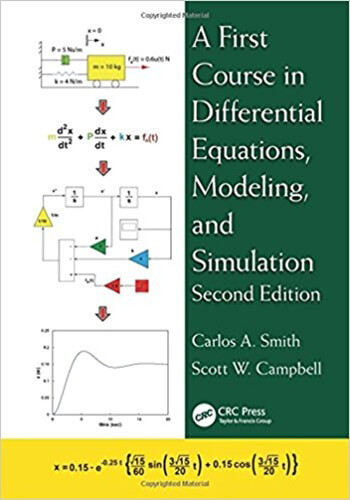
Product Details:
ISBN-13: 978-1482257229
Author: Carlos A. Smith (Author), Scott W. Campbell (Author)
A First Course in Differential Equations, Modeling, and Simulation shows how differential equations arise from applying basic physical principles and experimental observations to engineering systems. Avoiding overly theoretical explanations, the textbook also discusses classical and Laplace transform methods for obtaining the analytical solution of differential equations. In addition, the authors explain how to solve sets of differential equations where analytical solutions cannot easily be obtained.
Incorporating valuable suggestions from mathematicians and mathematics professors, the Second Edition:
- Expands the chapter on classical solutions of ordinary linear differential equations to include additional methods
- Increases coverage of response of first- and second-order systems to a full, stand-alone chapter to emphasize its importance
- Includes new examples of applications related to chemical reactions, environmental engineering, biomedical engineering, and biotechnology
- Contains new exercises that can be used as projects and answers to many of the end-of-chapter problems
- Features new end-of-chapter problems and updates throughout
Thus, A First Course in Differential Equations, Modeling, and Simulation, Second Edition provides students with a practical understanding of how to apply differential equations in modern engineering and science.
Table of Content:
- 1.1 An Introductory Example
- FIGURE 1.1 Mixing tank.
- FIGURE 1.2 Response of level in tank.
- 1.2 Differential Equations
- 1.2.1 Initial and Boundary Conditions
- FIGURE 1.3 Graph of Equation 1.18.
- FIGURE 1.4 RLC circuit.
- 1.2.2 Ordinary and Partial Differential Equations
- FIGURE 1.5 Well-insulated pipe.
- 1.3 Modeling
- 1.4 Forcing Functions
- FIGURE 1.6 Step change in flow of stream 1.
- FIGURE 1.7 Forcing function for Example 1.1.
- Example 1.1
- Example 1.2
- FIGURE 1.8 Forcing function for Example 1.2.
- Example 1.3
- Example 1.4
- 1.5 Book Objectives
- 1.6 Summary
- PROBLEMS
- FIGURE P1.1 Graphs for Problem 1.1.
- FIGURE P1.2 Thrust curve for a model rocket engine.
- 2 Objects in a Gravitational Field
- 2.1 An Example
- FIGURE 2.1 Object held aboveground.
- 2.2 Antidifferentiation: Technique for Solving First-Order Ordinary Differential Equations
- 2.3 Back to Section 2.1
- 2.4 Another Example
- 2.5 Separation of Variables: Technique for Solving First -Order Ordinary Differential Equations
- 2.6 Back to Section 2.4
- 2.7 Equations, Unknowns, and Degrees of Freedom
- 2.8 Partial Fraction Expansion
- 2.8.1 Unrepeated Real Roots
- 2.8.2 Repeated Real Roots
- Example 2.1
- Example 2.2
- 2.9 Summary
- PROBLEMS
- 3 Classical Solutions of Ordinary Linear Differential Equations
- 3.1 Examples of Differential Equations
- 3.1.1 Bioengineering: Chapter 8
- 3.1.2 Mechanical Translational: Chapter 6
- 3.1.3 Fluid System: Chapter 8
- FIGURE 3.1 Mass–spring–dashpot system.
- FIGURE 3.2 Liquid level.
- 3.1.4 Thermal System: Chapter 9
- FIGURE 3.3 Heat transfer from the sole plate of an electric iron.
- 3.1.5 Electrical Circuit: Chapter 10
- FIGURE 3.4 Electrical circuit.
- 3.2 Definition of a Linear Differential Equation
- Example 3.1
- 3.3 Integrating Factor Method
- Example 3.2
- Example 3.3
- Example 3.4
- 3.3.1 Development of the Integrating Factor Method
- 3.4 Solution of Homogeneous Differential Equations
- 3.4.1 Characteristic Equation
- Example 3.5
- 3.4.2 Roots of the Characteristic Equation
- DEVELOPMENT OF EQUATION 3.25
- 3.4.3 Qualitative System Response
- FIGURE 3.5 Roots of characteristic equation.
- Example 3.6
- Example 3.7
- 3.5 Solution of Nonhomogeneous Differential Equations
- 3.5.1 Homogeneous Solution (Natural Response) and Nonhomogeneous Solution (Forced Response)
- 3.5.2 Undetermined Coefficients
- TABLE 3.1 Solutions for the Particular Solution
- Example 3.8
- Example 3.9
- Example 3.10
- Example 3.11
- Example 3.12
- Example 3.13
- Example 3.14
- Example 3.15
- 3.5.3 Multiple Forcing Functions
- FIGURE 3.6 Cart with multiple forcing functions.
- 3.6 Variation of Parameters
- 3.6.1 Second-Order Systems
- Example 3.16
- Example 3.17
- Example 3.18
- CRAMER’S RULE
- 3.6.2 Higher-Order Systems
- 3.7 Handling Nonlinearities and Variable Coefficients
- 3.7.1 Taylor Series
- Example 3.19
- 3.7.2 Linearization of Nonlinear Differential Equations
- FIGURE 3.7 Linear approximation.
- Example 3.20
- FIGURE 3.8 Comparison of actual and linearized models.
- FIGURE 3.9 Comparison of actual and new linearized models.
- Example 3.21
- Example 3.22
- FIGURE 3.10 Comparison of actual and linearized models.
- FIGURE 3.11 Comparison of actual and linearized models.
- 3.8 Transient and Final Responses
- FIGURE 3.12 Graphs of (a) Equation 3.41 and (b) Equation 3.49.
- 3.9 Summary
- PROBLEMS
- FIGURE P3.1 Roots for Problem 3.6
- FIGURE P3.2 Water treatment basins for Problem 3.8.
- FIGURE P3.3 Spring–mass–dashpot system for Problem 3.11.
- FIGURE P3.4 Spring–mass–dashpot system for Problem 3.14.
- FIGURE P3.5 Mechanical system for Problem 3.16.
- FIGURE P3.6 Mechanical system for Problem 3.17.
- FIGURE P3.7 Mechanical system for Problem 3.18.
- FIGURE P3.8 Mechanical system for Problem 3.19.
- FIGURE P3.9 Electrical circuit for Problem 3.20.
- FIGURE P3.10 Electrical circuit for Problem 3.21.
- FIGURE P3.11 Electrical circuit for Problem 3.22.
- FIGURE P3.12 Electrical circuit for Problem 3.25.
- FIGURE P3.13 Electrical circuit for Problem 3.26.
- FIGURE P3.14 Electrical circuit for Problem 3.27.
- 4 Laplace Transforms
- 4.1 Definition of the Laplace Transform
- Example 4.1
- FIGURE 4.1 Common input signals: (a) unit step function, (b) pulse, (c) unit impulse function, and (d) sine wave.
- TABLE 4.1 Laplace Transforms of Common Functions
- 4.2 Properties and Theorems of the Laplace Transform
- 4.2.1 Linearity Property
- 4.2.2 Real Differentiation Theorem
- 4.2.3 Real Integration Theorem
- 4.2.4 Real Translation Theorem
- FIGURE 4.2 Function delayed in time is zero for all times less than the time delay t0.
- 4.2.5 Final Value Theorem
- 4.2.6 Complex Differentiation Theorem
- 4.2.7 Complex Translation Theorem
- 4.2.8 Initial Value Theorem
- Example 4.2
- Example 4.3
- Example 4.4
- 4.3 Solution of Differential Equations Using Laplace Transform
- 4.3.1 Inversion by Partial Fraction Expansion
- 4.3.1.1 Unrepeated Real Roots
- Example 4.5
- 4.3.1.2 Repeated Real Roots
- Example 4.6
- 4.3.1.3 Complex Roots
- 4.3.1.3.1 First-Order Expansion
- 4.3.1.3.2 Second-Order Expansion
- COMPLETING THE SQUARE
- Example 4.7
- Example 4.8
- Example 4.9
- Example 4.10
- Example 4.11
- Example 4.12
- Example 4.13
- Example 4.14
- Example 4.15
- 4.3.2 Handling Time Delays
- Example 4.16
- FIGURE 4.3 Input functions for Example 4.16. (a) Delayed unit step, u(t − 1). (b) Staircase of unit steps.
- 4.4 Transfer Functions
- 4.5 Algebraic Manipulations Using Laplace Transforms
- FIGURE 4.4 Frictionless carts with an external force.
- 4.6 Deviation Variables
- FIGURE 4.5 Mass–spring–dashpot system.
- Example 4.17
- Example 4.18
- FIGURE 4.6 Electrical circuit.
- 4.7 Summary
- PROBLEMS
- 5 Response of First- and Second-Order Systems
- 5.1 First-Order Systems
- 5.1.1 Step Function Input
- FIGURE 5.1 Response of a first-order system to a step change in input.
- TABLE 5.1 First-Order Step Response
- 5.1.2 Sinusoidal Function Input
- 5.1.3 Transfer Function
- 5.2 Second-Order Systems
- 5.2.1 Step Function Input
- 5.2.1.1 Types of Stable Systems
- FIGURE 5.2 Response of second-order system to a step change in forcing function.
- 5.2.1.2 Underdamped Response
- FIGURE 5.3 Second-order underdamped response (ζ = 0.5) of step input.
- TABLE 5.2 Second-Order Underdamped Step Response
- FIGURE 5.4 Effect of damping ratio on the second-order underdamped step response.
- FIGURE 5.5 Undamped response.
- 5.2.1.3 Undamped Response
- 5.2.2 Sinusoidal Function Input
- 5.2.3 Transfer Function
- 5.3 Examples
- FIGURE 5.6 Mass–spring–dashpot system.
- Example 5.1
- Example 5.2
- FIGURE 5.7 Electrical circuit.
- Example 5.3
- FIGURE 5.8 Information for Example 5.3.
- Example 5.4
- FIGURE 5.9 Information for Example 5.4.
- 5.4 Some Concluding Remarks
- 5.5 Summary
- PROBLEMS
- FIGURE P5.1 Schematic for Problem 5.1.
- FIGURE P5.2 Electrical circuit for Problem 5.2.
- FIGURE P5.3 Information for Problem 5.3.
- FIGURE P5.4 Mechanical system for Problem 5.7.
- 6 Mechanical Systems: Translational
- 6.1 Mechanical Law, System Components, and Forces
- 6.1.1 Mechanical Law
- FIGURE 6.1 Springs.
- 6.1.2 System Components
- 6.1.2.1 Springs
- FIGURE 6.2 Forces generated by springs.
- FIGURE 6.3 (a) Ideal and (b) real springs.
- 6.1.2.2 Dashpots (Pistons or Dampers)
- FIGURE 6.4 Spring–mass system showing dashpot.
- 6.1.2.3 Ideal Pulley
- FIGURE 6.5 Mechanical system showing a pulley.
- FIGURE 6.6 (a) Dry friction force between two surfaces. (b) Fluid friction force between two surfaces.
- 6.1.3 Forces
- FIGURE 6.7 Demonstration of the negative sign in Equation 6.4.
- 6.2 Types of Systems
- 6.2.1 Undamped System
- FIGURE 6.8 Mass–spring system.
- FIGURE 6.9 Response for undamped system—with and without resonance.
- 6.2.2 Damped System
- FIGURE 6.10 Spring–mass system.
- 6.3 D’Alembert’s Principle and Free Body Diagrams
- FIGURE 6.11 Mass–spring–dashpot system.
- FIGURE 6.12 Free body diagram of the system shown in Figure 6.11.
- FIGURE 6.13 Response of cart shown in Figure 6.11.
- 6.4 Examples
- FIGURE 6.14 System consisting of two blocks.
- FIGURE 6.15 Displacement of blocks after applying force.
- Example 6.1
- FIGURE 6.16 Frictionless carts with an external force.
- FIGURE 6.17 Response of carts.
- FIGURE 6.18 Free body diagrams for carts in Figure 6.16.
- FIGURE 6.19 Free body diagrams for carts in Figure 6.16.
- Example 6.2
- FIGURE 6.20 Cart with friction and an external force.
- FIGURE 6.21 Free body diagrams for carts of Figure 6.20.
- FIGURE 6.22 Free body diagrams for carts of Figure 6.20.
- Example 6.3
- FIGURE 6.23 Two blocks with friction.
- 6.5 Vertical Systems
- Example 6.4
- FIGURE 6.24 Vertical mechanical system.
- FIGURE 6.25 Displacement of system of Example 6.4.
- 6.6 Summary
- PROBLEMS
- FIGURE P6.1 Mechanical system for Problem 6.1.
- FIGURE P6.2 Mechanical system for Problem 6.2.
- FIGURE P6.3 Mechanical system for Problem 6.3.
- FIGURE P6.4 Mechanical system for Problem 6.4.
- FIGURE P6.5 Mechanical system for Problem 6.5.
- FIGURE P6.6 Mechanical system for Problem 6.6.
- FIGURE P6.7 Mechanical system for Problem 6.7.
- FIGURE P6.8 Mechanical system for Problem 6.8.
- FIGURE P6.9 Mechanical system for Problem 6.9.
- FIGURE P6.10 Mechanical system for Problem 6.10.
- FIGURE P6.11 Mechanical system for Problem 6.11.
- FIGURE P6.12 Mechanical system for Problem 6.12.
- FIGURE P6.13 Mechanical system for Problem 6.13.
- FIGURE P6.14 Mechanical system for Problem 6.14.
- FIGURE P6.15 Mechanical system for Problem 6.15.
- FIGURE P6.16 Mechanical system for Problem 6.16.
- FIGURE P6.17 Mechanical system for Problem 6.17.
- FIGURE P6.18 Cart system for Problem 6.18.
- FIGURE P6.19 Block system for Problem 6.19.
- FIGURE P6.20 Block system for Problem 6.20.
- FIGURE P6.21 Block system for Problem 6.21.
- FIGURE P6.22 Block system for Problem 6.22.
- 7 Mechanical Systems: Rotational
- 7.1 Mechanical Law, Moment of Inertia, and Torque
- FIGURE 7.1 Angular position θ.
- TABLE 7.1 Analogous Relations between Translational and Rotational Systems
- 7.1.1 Mass Moment of Inertia
- Example 7.1
- FIGURE 7.2 Rotation of a slender bar and enlarged view of volume element.
- 7.1.2 Torque
- Example 7.2
- FIGURE 7.3 Moment arm d between axis of rotation A and the line of action C of a force F.
- FIGURE 7.4 A pendulum comprised of a slender rod.
- FIGURE 7.5 Moment arm evaluation (a) and free body diagram (b) for the pendulum of Example 7.2.
- FIGURE 7.6 Comparison of analytical solution of linearized Equation 7.20 to numerical solution of Equation 7.17 for (a) θ0 = 30° and (b) θ0 = 90°.
- 7.2 Torsion Springs
- FIGURE 7.7 Torsion bar.
- Example 7.3
- FIGURE 7.8 System of two rotating masses and two torsion springs.
- FIGURE 7.9 Free body diagrams of the masses in Example 7.3.
- 7.3 Rotational Damping
- FIGURE 7.10 Damping in a rotational system.
- Example 7.4
- FIGURE 7.11 Rotational system of Example 7.4.
- FIGURE 7.12 Free body diagrams for Example 7.4.
- FIGURE 7.13 Solution to Equations 7.32 and 7.33 using parameters given in part (b).
- 7.4 Gears
- FIGURE 7.14 (a) Two gears and (b) partial FBD showing the contact force fC.
- Example 7.5
- FIGURE 7.15 Geared elements of Example 7.5.
- FIGURE 7.16 Free body diagrams for the gears of Example 7.5.
- 7.5 Systems with Rotational and Translational Elements
- Example 7.6
- FIGURE 7.17 Drum and mass system of Example 7.6.
- FIGURE 7.18 Free body diagrams for Example 7.6.
- FIGURE 7.19 Velocity (a) and spring stretch (b) versus time for the system of Example 7.6.
- 7.6 Summary
- PROBLEMS
- FIGURE P7.1 Disks of mass m, radius R, and length L for parts (a) and (b) and the suggested volume element.
- FIGURE P7.2 Pendulum made of a slender bar with friction at the pin.
- FIGURE P7.3 Torsion spring with damping.
- FIGURE P7.4 Single torsion spring of Problem 7.4.
- FIGURE P7.5 Wheel and pulley system of Problem 7.5.
- FIGURE P7.6 Viscous coupler.
- FIGURE P7.7 Centrifugal clutch.
- FIGURE P7.8 Viscous coupler of Problem 7.8.
- FIGURE P7.9 System of two masses and torsion springs for Problem 7.9.
- FIGURE P7.10 Mass and rotating drum of Problem 7.10.
- FIGURE P7.11 System of translating and rotating masses of Problem 7.11.
- FIGURE P7.12 System of Problem 7.12.
- FIGURE P7.13 Single-speed bicycle.
- FIGURE P7.14 Scotch yoke linkage.
- FIGURE P7.15 Winch of Problem 7.15.
- FIGURE P7.16 Spool transfer system of Problem 7.16.
- FIGURE P7.17 Disk and two masses of Problem 7.17.
- FIGURE P7.18 System of Problem 7.18.
- 8 Mass Balances
- 8.1 Conservation of Mass
- FIGURE 8.1 Generic system.
- 8.1.1 Multicomponent Systems
- 8.1.2 Types of Processes
- 8.2 Flow Rates and Concentrations
- 8.3 Elements and Experimental Facts
- 8.3.1 Flow Element
- FIGURE 8.2 Process valve.
- FIGURE 8.3 Control valve.
- 8.3.2 Liquid Service
- FIGURE 8.4 Liquid level.
- 8.3.3 Gas Service
- 8.4 Examples
- Example 8.1
- Example 8.2
- FIGURE 8.5 Mixing tank.
- Example 8.3
- Example 8.4
- FIGURE 8.6 Gas system.
- 8.5 Expressions for Mass Transport and Chemical Reactions
- 8.5.1 Mass Transport
- FIGURE 8.7 Mass transfer of component A from phase I to phase II.
- 8.5.2 Chemical Reactions
- FIGURE 8.8 Chemical reactor.
- 8.5.2.1 Half-Life
- 8.5.3 Batch Processes
- FIGURE 8.9 Closed system.
- 8.5.3.1 Batch Separation
- FIGURE 8.10 Batch reactor.
- 8.5.3.2 Batch Reactor
- 8.6 Additional Examples
- Example 8.5
- FIGURE 8.11 Water treatment basins.
- Example 8.6
- FIGURE 8.12 Benzene concentration in basins.
- Example 8.7
- FIGURE 8.13 Batch reactor for Example 8.7.
- Example 8.8
- FIGURE 8.14 Water filter.
- 8.7 Application to Bioengineering Processes
- FIGURE 8.15 Body divided into compartments for modeling purposes.
- 8.7.1 Compartmental Modeling
- FIGURE 8.16 Disappearance of a protein (solute) in blood.
- FIGURE 8.17 Transfer of a solute between two compartments.
- 8.7.2 Biological Reactions
- Example 8.9
- FIGURE 8.18 Single compartment for Example 8.9.
- Example 8.10
- FIGURE 8.19 Response of an antibiotic.
- Example 8.11
- FIGURE 8.20 Antibiotic in blood.
- 8.7.3 Fermentation
- FIGURE 8.21 Substrate concentration versus time.
- Example 8.12
- Example 8.13
- 8.8 Final Comments
- 8.9 Summary
- References
- PROBLEMS
- FIGURE P8.1 Tank for Problem 8.1.
- FIGURE P8.2 Process for Problem 8.2.
- FIGURE P8.3 Tank for Problem 8.3.
- FIGURE P8.4 Tank for Problem 8.4.
- FIGURE P8.5 Tanks for Problem 8.5.
- FIGURE P8.6 Tank for Problem 8.9.
- FIGURE P8.7 Mixing tank for Problem 8.10.
- Steady-State Values
- FIGURE P8.8 Tank system for Problem 8.11.
- FIGURE P8.9 Storage tank for Problem 8.14.
- FIGURE P8.10 Tray of a distillation column for Problem 8.15.
- FIGURE P8.11 Process tank with pump manipulating exit stream.
- FIGURE P8.12 Compartments representing muscle and blood.
- FIGURE P8.13 Chemical hood for Problem 8.25.
- 9 Thermal Systems
- 9.1 Conservation of Energy
- 9.2 Modes of Heat Transfer
- 9.3 Conduction
- FIGURE 9.1 Heat conduction through a plate.
- 9.4 Convection
- FIGURE 9.2 Convection of heat from an object of surface temperature T and surface area A to a fluid at temperature Tf.
- 9.5 Conduction and Convection in Series
- FIGURE 9.3 Heat transfer by convection and conduction.
- 9.6 Accumulated or Stored Energy
- 9.7 Some Examples
- Example 9.1: Convective Heat Transfer
- FIGURE 9.4 Graph of Equation 9.26 with two different values of α.
- Example 9.2: Heating of a Liquid in a Jacketed, Stirred Vessel
- FIGURE 9.5 Heating of water in a jacketed, stirred vessel.
- Example 9.3: Convective Heat Transfer with Internal Generation
- FIGURE 9.6 Heat transfer from the sole plate of an electric iron.
- FIGURE 9.7 Temperature profile for the sole plate showing ultimate temperature and time to reach 100°C.
- 9.8 Heat Transfer in a Flow System
- FIGURE 9.8 Heating of a vessel with inlet and outlet flows.
- Example 9.4: Heating of a Vessel with Inflows and Outflows
- 9.9 Thermal Effects in a Reactive System
- FIGURE 9.9 Solution to Equations 9.75 and 9.76 for an adiabatic batch reactor using given parameter values.
- 9.10 Boundary Value Problems in Heat Transfer
- Example 9.5: Temperature Profile and Heat Flow in Wire Insulation
- FIGURE 9.10 An insulated wire.
- FIGURE 9.11 Expanded view of the insulation showing the chosen volume element.
- Example 9.6: Steady-State Temperature Profile in a Sphere with Internal Heat Generation
- FIGURE 9.12 Spherical pellet and selected volume element.
- FIGURE 9.13 Temperature versus radial position for the sphere of Example 9.6. The lumped parameter approximation is represented by the solid line and the full solutions by the dashed curves. The long dashes, medium dashes, and short dashes correspond to Biot numbers of 1.0, 0.1, and 0.02, respectively.
- Example 9.7: Steady-State Heat Transfer from an Extended Surface
- FIGURE 9.14 Heat transfer from an extended surface.
- FIGURE 9.15 Percent difference between the heat flow from an extended, infinitely long circular rod calculated assuming two-dimensional conduction and that calculated assuming one-dimensional conduction.
- 9.11 Summary
- PROBLEMS
- FIGURE P9.1 Cooled water bath of Problem 9.8.
- FIGURE P9.2 Heated bath of Problem 9.9.
- 10 Electrical Systems
- 10.1 Some Definitions and Conventions
- FIGURE 10.1 Schematic of ideal voltage and current sources.
- 10.2 Electrical Laws, Components, and Initial Conditions
- 10.2.1 Electrical Laws
- FIGURE 10.2 Closed-loop electrical circuit.
- FIGURE 10.3 Electrical node.
- 10.2.2 Electrical Components
- FIGURE 10.4 Resistor.
- FIGURE 10.5 Capacitor.
- FIGURE 10.6 Tank with flexible membrane.
- FIGURE 10.7 Capacitor becoming an open circuit at steady state.
- FIGURE 10.8 Inductor.
- FIGURE 10.9 Inductor becoming a simple conductor at steady state.
- 10.2.3 Initial Conditions
- FIGURE 10.10 Electrical circuit.
- FIGURE 10.11 Voltage and current behavior.
- 10.3 Examples of Electrical Circuits
- Example 10.1
- FIGURE 10.12 RC circuit.
- FIGURE 10.13 RC circuit at initial steady state.
- FIGURE 10.14 Response of RC circuit shown in Figure 10.12.
- Example 10.2
- FIGURE 10.15 RL circuit.
- FIGURE 10.16 RL circuit at initial steady state.
- Example 10.3
- FIGURE 10.17 RLC circuit.
- Example 10.4
- FIGURE 10.18 Circuit for Example 10.4.
- FIGURE 10.19 Circuit for Example 10.4, part (a).
- FIGURE 10.20 Circuit for Example 10.4, part (b).
- 10.3.1 Undamped Circuit (Natural Frequency and Resonance)
- FIGURE 10.21 LC circuits.
- FIGURE 10.22 Responses of LC circuits.
- FIGURE 10.23 LC circuits with some amount of resistance.
- 10.4 Additional Examples
- Example 10.5
- FIGURE 10.24 Electrical circuit for Example 10.5.
- Example 10.6
- FIGURE 10.25 Electrical circuit for Example 10.6.
- FIGURE 10.26 Electrical circuit for Example 10.6 showing open circuit.
- NODAL METHOD
- FIGURE 10.27 Electrical circuit showing information for the nodal method.
- MESH METHOD
- FIGURE 10.28 Electric circuit showing meshes.
- Example 10.7
- FIGURE 10.29 Electrical circuit.
- FIGURE 10.30 Redraw of Figure 10.29.
- FIGURE 10.31 Redraw of Figure 10.30.
- Example 10.8
- FIGURE 10.32 Circuits for Example 10.8.
- FIGURE 10.33 Charging and discharging of the capacitor in Figure 10.29a.
- 10.5 Energy and Power
- FIGURE 10.34 Electrical component.
- 10.5.1 Resistors
- FIGURE 10.35 Resistor.
- 10.5.2 Capacitors
- 10.5.3 Inductors
- Example 10.9
- FIGURE 10.36 RLC circuit.
- FIGURE 10.37 Power and energy responses of components in Figure 10.36.
- FIGURE 10.38 Circuits for t ≥ 2 s.
- FIGURE 10.39 Voltages and currents for circuits in Figure 10.36.
- FIGURE 10.40 Energy contained in the circuits of Figure 10.38.
- Example 10.10
- FIGURE 10.41 Electrical circuit.
- FIGURE 10.42 Chip temperature.
- 10.6 RC Circuits as Filters
- FIGURE 10.43 Ideal filters. (a) High-pass filter. (b) Low-pass filter.
- FIGURE 10.44 RC circuit.
- 10.6.1 High-Pass Filter
- FIGURE 10.45 Voltage drop across a resistor in an RC circuit.
- FIGURE 10.46 Performance of an RC circuit as a high-pass filter.
- 10.6.2 Low-Pass Filter
- FIGURE 10.47 Voltage drop across a capacitor in an RC circuit.
- FIGURE 10.48 Performance of an RC circuit as a low-pass filter.
- FIGURE 10.49 Performance of an RC circuit as a low-pass filter and as a high-pass filter. (a) Input signal to circuit. (b) Output of high-pass filter. (c) Output of low-pass filter.
- 10.7 Summary
- PROBLEMS
- FIGURE P10.1 Circuit for Problem 10.1.
- FIGURE P10.2 Circuit for Problem 10.2.
- FIGURE P10.3 Circuit for Problem 10.3.
- FIGURE P10.4 Circuit for Problem 10.4.
- FIGURE P10.5 Circuit for Problem 10.5.
- FIGURE P10.6 Circuit for Problem 10.6.
- FIGURE P10.7 Circuit for Problem 10.7.
- FIGURE P10.8 Circuit for Problem 10.8.
- FIGURE P10.9 Circuit for Problem 10.9.
- FIGURE P10.10 Circuit for Problem 10.10.
- FIGURE P10.11 Circuit for Problem 10.11.
- FIGURE P10.12 Circuit for Problem 10.12.
- FIGURE P10.13 Circuit for Problem 10.13.
- FIGURE P10.14 Circuit for Problem 10.14.
- FIGURE P10.15 Circuit for Problem 10.15.
- FIGURE P10.16 Circuit for Problem 10.16.
- FIGURE P10.17 Circuit for Problem 10.17.
- FIGURE P10.18 Circuit for Problem 10.18.
- FIGURE P10.19 Circuit for Problem 10.19.
- FIGURE P10.20 Circuit for Problem 10.20.
- FIGURE P10.21 Circuit for Problem 10.21.
- FIGURE P10.22 Circuit for Problem 10.22.
- FIGURE P10.23 Circuit for Problem 10.23.
- FIGURE P10.24 Circuit for Problem 10.24.
- FIGURE P10.25 Circuit for Problem 10.25.
- FIGURE P10.26 Circuit for Problem 10.26.
- FIGURE P10.27 (a) Circuit for Problem 10.27a. (b) Circuit for Problem 10.27b.
- FIGURE P10.28 Circuit for Problem 10.28.
- 11 Numerical Simulation
- 11.1 Numerical Solution of Differential Equations
- TABLE 11.1 Numerical Solution of Equation 11.1 for Tf = 200, T0 = 25, and α = 0.1
- 11.2 Euler’s Method for First-Order Ordinary Differential Equations
- Example 11.1
- 11.3 Euler’s Method for Second-Order Ordinary Differential Equations
- Example 11.2
- 11.4 Step Size
- FIGURE 11.1 Illustration of the effect of step size in Euler’s method using the differential equation of Example 11.1.
- 11.5 More Sophisticated Methods
- 11.6 Representation of Differential Equations by Block Diagrams
- 11.6.1 Basic Blocks
- 11.6.2 Guidelines for Constructing Block Diagrams
- Example 11.3
- 11.6.3 Some Additional Examples
- Example 11.4
- Example 11.5
- Example 11.6
- 11.6.4 Some Additional Source Blocks
- 11.6.4.1 Step Block
- 11.6.4.2 Sine Wave
- 11.7 Additional Examples
- Example 11.7
- FIGURE 11.2 Diagram for the simulation of Equations 6.36 and 6.37.
- FIGURE 11.3 Response of the carts of Example 11.7.
- FIGURE 11.4 Difference (%) between the responses obtained from the analytical solution and simulation. (a) Cart 1 and (b) Cart 2.
- Example 11.8
- FIGURE 11.5 Block diagram for the simulation of Equation 8.32.
- FIGURE 11.6 Response of the level in the tank.
- FIGURE 11.7 Response of the level to three consecutive changes in inlet flow of 2 m3/min.
- Example 11.9
- FIGURE 11.8 Electrical circuit.
- FIGURE 11.9 Simulation (block diagram) of Equation 11.22b.
- FIGURE 11.10 Response of voltage drop vD.
- FIGURE 11.11 Block diagram for Equations 11.17 through 11.21.
- 11.8 Summary
- Reference
- PROBLEMS
- FIGURE P11.1 Thrust curve for rocket engine of Problem 11.10.
- FIGURE P11.2 Shock absorber of Problem 11.15.
- FIGURE P11.3 Speed bump of Problem 11.15.
- FIGURE P11.4 Mechanical system for Problem 11.17.
- FIGURE P11.5 Mechanical system for Problem 11.18.
- FIGURE P11.6 Waste disposal tank with three pumps.
- Back Matter
- Answers to Selected Problems
- Chapter 1
- Chapter 2
- Chapter 3
- Chapter 4
- Chapter 5
- Chapter 6
- Chapter 7
- Chapter 8
- Chapter 9
- Chapter 10
- Chapter 11
- Index
People Also Search:
first course in differential equations modeling and simulation
first course in differential equations modeling and simulation 2nd smith
first course in differential equations modeling and simulation 2nd smith download scribd
first course in differential equations modeling and simulation 2nd smith solution manual download pdf
Related products
Solution Manual
Solution Manual
Solution manual for Accounting: Tools for Business Decision Making Kimmel Weygandt Kieso 5th Edition
Solution Manual
Solution Manual
Solution Manual
Solution Manual
Solution Manual for Introduction to Robotics Mechanics and Control 3rd Edition by Craig


